Fourier Series
A Fourier series decomposes a periodic function or periodic signal into a sum of simple oscillating functions, namely sines and cosines (or complex exponentials).
In this section, ƒ(x) denotes a function of the real variable x. This function is usually taken to be periodic, of period 2π, which is to say that ƒ(x + 2π) = ƒ(x), for all real numbers x. We will attempt to write such a function as an infinite sum, or series of simpler 2π–periodic functions. We will start by using an infinite sum of sine and cosine functions on the interval [−π, π], as Fourier did (see the quote above), and we will then discuss different formulations and generalizations.
Fourier's formula for 2π-periodic functions using sines and cosines
For a 2π-periodic function ƒ(x) that is integrable on [−π, π], the numbers
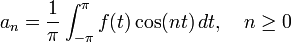
and
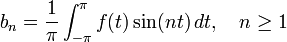
are called the Fourier coefficients of ƒ. One introduces the partial sums of the Fourier series for ƒ, often denoted by
![(S_N f)(x) = \frac{a_0}{2} + \sum_{n=1}^{N} \, [a_n \cos(nx) + b_n \sin(nx)], \quad N \ge 0.](http://upload.wikimedia.org/math/2/d/a/2da2b0202fe9610a121f2318886417a7.png)
The partial sums for ƒ are trigonometric polynomials. One expects that the functions SN ƒ approximate the function ƒ, and that the approximation improves as N tends to infinity. The infinite sum
![\frac{a_0}{2} + \sum_{n=1}^{\infty} \, [a_n \cos(nx) + b_n \sin(nx)]](http://upload.wikimedia.org/math/b/1/7/b179dd8b9ec47ca2a158864182d64264.png)
is called the Fourier series of ƒ.
The Fourier series does not always converge, and even when it does converge for a specific value x0 of x, the sum of the series at x0 may differ from the value ƒ(x0) of the function. It is one of the main questions in Harmonic analysis to decide when Fourier series converge, and when the sum is equal to the original function. If a function is square-integrable on the interval [−π, π], then the Fourier series converges to the function at almost every point. In engineering applications, the Fourier series is generally presumed to converge everywhere except at discontinuities, since the functions encountered in engineering are more well behaved than the ones that mathematicians can provide as counter-examples to this presumption. In particular, the Fourier series converges absolutely and uniformly to ƒ(x) whenever the derivative of ƒ(x) (which may not exist everywhere) is square integrable.[2] See Convergence of Fourier series.
It is possible to define Fourier coefficients for more general functions or distributions, in such cases convergence in norm or weak convergence is usually of interest.
Example: a simple Fourier series

We now use the formulae above to give a Fourier series expansion of a very simple function. Consider a sawtooth function


In this case, the Fourier coefficients are given by

It can be proved that the Fourier series converges to ƒ(x) at every point x where ƒ is differentiable, and therefore:
-
![\begin{align} f(x) &= \frac{a_0}{2} + \sum_{n=1}^{\infty}\left[a_n\cos\left(nx\right)+b_n\sin\left(nx\right)\right] \\ &=2\sum_{n=1}^{\infty}\frac{(-1)^{n+1}}{n} \sin(nx), \quad \mathrm{for} \quad x - \pi \notin 2 \pi \mathbf{Z}. \end{align}](http://upload.wikimedia.org/math/c/0/6/c06c0f50fec40edaf0ab2eb64841e9bf.png)
(
When x = π, the Fourier series converges to 0, which is the half-sum of the left- and right-limit of ƒ at x = π. This is a particular instance of the Dirichlet theorem for Fourier series.
One notices that the Fourier series expansion of our function looks much less simple than the formula ƒ(x) = x, and so it is not immediately apparent why one would need this Fourier series. While there are many applications, we cite Fourier's motivation of solving the heat equation. For example, consider a metal plate in the shape of a square whose side measures π meters, with coordinates (x, y) ∈ [0, π] × [0, π]. If there is no heat source within the plate, and if three of the four sides are held at 0 degrees Celsius, while the fourth side, given by y = π, is maintained at the temperature gradient T(x, π) = x degrees Celsius, for x in (0, π), then one can show that the stationary heat distribution (or the heat distribution after a long period of time has elapsed) is given by
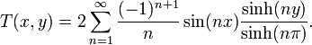
Here, sinh is the hyperbolic sine function. This solution of the heat equation is obtained by multiplying each term of Eq.1 by sinh(ny)/sinh(nπ). While our example function f(x) seems to have a needlessly complicated Fourier series, the heat distribution T(x, y) is nontrivial. The function T cannot be written as a closed-form expression. This method of solving the heat problem was only made possible by Fourier's work.
Another application of this Fourier series is to solve the Basel problem by using Parseval's theorem. The example generalizes and one may compute ζ(2n), for any positive integer n.
Exponential Fourier series
We can use Euler's formula,
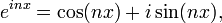
where i is the imaginary unit, to give a more concise formula:

The Fourier coefficients are then given by:
The Fourier coefficients an, bn, cn are related via

and

The notation cn is inadequate for discussing the Fourier coefficients of several different functions. Therefore it is customarily replaced by a modified form of ƒ (in this case), such as F or  and functional notation often replaces subscripting. Thus:
![\begin{align} f(x) &= \sum_{n=-\infty}^{\infty} \hat{f}(n)\cdot e^{inx} \\ &= \sum_{n=-\infty}^{\infty} F[n]\cdot e^{inx} \quad \mbox{(engineering)}. \end{align}](http://upload.wikimedia.org/math/4/0/4/404d6e7a78b18521aa2d32f6c70240fd.png)
In engineering, particularly when the variable x represents time, the coefficient sequence is called a frequency domain representation. Square brackets are often used to emphasize that the domain of this function is a discrete set of frequencies.
Fourier series on a general interval [a, b]
The following formula, with appropriate complex-valued coefficients G[n], is a periodic function with period τ on all of R:
![g(x)=\sum_{n=-\infty}^\infty G[n]\cdot e^{i 2\pi \frac{n}{\tau} x}\ .](http://upload.wikimedia.org/math/a/1/7/a175791c6d1eb7b82bb2c32c5906b4fb.png)
If a function is square-integrable in the interval [a, a + τ], it can be represented in that interval by the formula above. If g(x) is integrable, then the Fourier coefficients are given by:
![G[n] = \frac{1}{\tau}\int_a^{a+\tau} g(x)\cdot e^{-i 2\pi \frac{n}{\tau} x}\, dx.](http://upload.wikimedia.org/math/6/1/a/61a37ec6e60114cc4c1c034156ad94b8.png)
Note that if the function to be represented is also τ-periodic, then a is an arbitrary choice. Two popular choices are a = 0, and a = −τ/2.
Another commonly used frequency domain representation uses the Fourier series coefficients to modulate a Dirac comb:
![G(f) \ \stackrel{\mathrm{def}}{=} \ \sum_{n=-\infty}^{\infty} G[n]\cdot \delta \left(f-\frac{n}{\tau}\right)](http://upload.wikimedia.org/math/e/c/5/ec5b15aee84257a616ce867656034901.png)
where variable ƒ represents a continuous frequency domain. When variable x has units of seconds, ƒ has units of hertz. The "teeth" of the comb are spaced at multiples (i.e. harmonics) of 1/τ, which is called the fundamental frequency. The original g(x) can be recovered from this representation by an inverse Fourier transform:
![\begin{align} \mathcal{F}^{-1}\{G(f)\} &= \mathcal{F}^{-1}\left\{ \sum_{n=-\infty}^{\infty} G[n]\cdot \delta \left(f-\frac{n}{\tau}\right)\right\}\\ &= \sum_{n=-\infty}^{\infty} G[n]\cdot \underbrace{\mathcal{F}^{-1}\left\{\delta\left(f-\frac{n}{\tau}\right)\right\}}_{e^{i2\pi \frac{n}{\tau} x}\cdot \underbrace{\mathcal{F}^{-1}\{\delta (f)\}}_{1}}\\ &= \sum_{n=-\infty}^{\infty} G[n]\cdot e^{i2\pi \frac{n}{\tau} x} \quad = \ \ g(x). \end{align}](http://upload.wikimedia.org/math/9/c/a/9cad761f48f4b08af25320026114f295.png)
The function  is therefore commonly referred to as a Fourier transform, even though the Fourier integral of a periodic function is not convergent.
출처 : www.wikipedia.org
'Physics' 카테고리의 다른 글
| Relationship between exponential and trigonometric functions (0) | 2010.12.08 |
|---|---|
| MATLAB Links (0) | 2010.12.06 |
| Partial Differential Equations in MATLAB (0) | 2010.12.06 |
| XRD Crystallite Size Calculator using Scherrer Formula (0) | 2010.12.01 |
| Shape factor (X-ray diffraction) (0) | 2010.12.01 |
| In-Phase & Quadrature Sinusoidal Components (0) | 2010.11.08 |
| Stephen Wolfram TED Talk 영상 (0) | 2010.10.27 |
| 주기율표(Periodic Table) (0) | 2010.10.26 |
| 깨달음 (0) | 2010.10.26 |
| Mathematica 참고사이트 (0) | 2010.10.23 |

